Introduction.

In this text, we are concerned with the process of "classification" or "taxonomy" and specifically with formal computer methods to assist us with this process. It is a very natural idea and one that we uuse constantly, often without realising what is happening. For example, we might overhear the following conversation in a greengrocer's shop.

"Which apples do you want ?"
"The green ones over there."

Here the speaker has performed a classification of the selection of apples offered for sale and has used the attributes "colour" and "position" to give a unique definition of the class of apples which he or she wants. If it was not sufficient to give a unique definition you might have the following additions:

"Do you mean these ?" pointing to one container of apples
"No, no. The ones on the lower shelf." giving a more accurate position.

Such a classification is typically carried out in seconds and only applies to one particular occasion. Next time you visit the same shop, they may have sold out of that particular variety or rearranged the display so that they occur in a totally different position.

If you think about it over the next day or two, you will realise how often this process is used in everyday conversation. A surname is used to identify all members of a particular family, a Faculty or degree and year to identify a particular group of students, and within this, a reference to a particular lecture course. All these classifications are used for particular reasons, for example the students attending a particular lecture course may need special treatment because they have a common problem or a need for some specialised facilities. A group of friends may think up a nickname by which they can refer to themselves instead of listing all their names every time they wish to make a comment about themselves (in its crudest form "us" as opposed to "them" or everyone else.)

When we come to transfer this process to a computer, there are several different criteria that must be considered. Firstly, putting data into the correct form for input to a computer and then typing it in, is a comparatively lengthy process and so we do not wish to repeat it unnecessarily. This means we need to use attributes which will apply for a considerable length of time. In the above example, we should need to learn the name of the variety (e.g. "Bramley" or "Granny Smith") rather than the position in which it was placed in the shop on a particular occasion.

Secondly the attributes must be expressed in terms the computer can handle, for example "medium size" would need to be defined as a breadth lying between two values specified in inches or millimetres.

Thirdly, the computer is not able to look at the overall picture and decide how much data is needed to specify the required class uniquely. Instead the criteria for division into classes have to be provided and can then be applied to many hundreds of objects, far more than a human could easily classify.

Classification Process.

The classification process is very widely used, and a number of distinct steps can be identified. Only the fourth and fifth steps can be carried out by means of computer programs.

1. Study a number of ‘objects’.
2. Define ‘attributes’ which describe them.
3. Measure these attributes for each object.
4. Use these values to define ‘classes’ or ‘taxa’.
5. Assign each object to a class or taxon. (Identification).

Types of Variable.

Variables are used to define the attributes and the type of variable will determine the accuracy of measurement and the possible forms of storage within the computer. Consider the following examples of data could relate to students within a group.

1. height in inches.
2. weight in pounds or kilogrammes.

These are examples of "Numeric Variables". They are real numbers and may be measured to as many decimal places as the equipment will permit. They are continuous and objective - the values should be the same whoever is taking the measurements. The ideas of distance and ordering apply to this type of data.

3. presence or absence from this class.
4. sex.
5. pleasant or unpleasant company.

These are "Binary Variables". They may take one of two values and may be coded as (0 or 1), (p or a), (y'or n) depending on the question. They are usually converted to 0/1 within a computer. Variables 3 and 4 are objective, there is not likely to any disagreement as to the sex of an individual or whether he or she is physically present at a given lecture. Variable 5 is highly subjective and may give as much information about the person answering the question as about the student being described. There is a danger that sociological surveys with a large number of yes/no questions may lead to highly subjective binary data.

6. age in years.

This an example of an "Ordered-multistate Variable", sometimes called an "Integer Variable". The values are integers and the data is usually objective. It is ordered in the same way as the positive integers are and the usual concepts of distance apply as they did for the numeric data.

7. colour of eyes.
8. colour of hair.
9. nationality.

These are examples of "Unordered-multistate Variables" or simply "Multistate Variables". The values may often be coded as single letters or numbers to save time on input and these may appear to imply an ordering of the data (if only ASCII values of the characters used), but the concepts of distance and ordering cannot be applied. It is meaningless to try and decide whether blue eyes are more similar to hazel or to brown, the only relevant question is whether two people have the same colour of eyes as each other or not. They are often subjective, just as the binary variables were and in some cases, such as nationality, may not even be single-valued.

The type of variable used for a particular attribute will dictate the accuracy of measurement, the appropriate tests for validity and the choice of similarity and distance coefficients available.

Causes of Invalid Taxa.

The most frequent cause of error in a taxonomy is due to carelessness or misunderstanding. A taxonomy is correctly defined for a small group of objects under a particular set of circumstances and works very well in this context. Word gets around that this particular taxonomer has a "good" taxonomy for these objects and others studying the same area come along and apply it, like a god-given revelation, to all objects under all conditions. This is quite unreasonable and I hope you will take care not to fall into this particular trap.

In this case, the taxonomy was valid for the original context. If any of the following causes apply, the resulting classification will never be valid and should be re-calculated.

1. The set of attributes is incomplete. The object is not fully described by the attributes which have been defined and, in particular, some which we instinctively use to split the objects into groups have been omitted.

2. The sample of objects used to define the taxonomy do not represent the total range of objects to be studied. This means that when we come to identify new objects, some will not fit into any of the groups defined in the classification.

3. Faulty measurement. e.g. carelessness leading to values being written down incorrectly.

4. Attributes not clearly defined. e.g. some height measurements recorded in inches and others in centimetres or all measurements are of height in inches, but some recorders take the measurement from bare-heels to the top of the head while others allow piled-up hairstyles and high-heels.

5. Inappropriate method of calculating similarity. Different types of variable require different ways of calculating similarity and the results will be meaningless if these are not matched up correctly.

6. Inappropriate method of calculating the clusters. The various methods of calculating clusters depend on certain assumptions about the data supplied to them and will give false and misleading results if these assumptions are not correct for the chosen set of data.

Terminology.

"Object", also called "individual" or "operational taxonomic unit" (usually abbreviated to OTU).

Whatever we are trying to classify. Strictly speaking these are themselves the result of a very crude taxonomy since an attempt to classify, say, animals will have start by dividing everything within reach into "animal" and "non-animal" (probably by some very crude criterion such as "if it moves it's an animal") and only take measurements of the animals.

"Attribute", also called "property" or "character".

Some aspect of the object which may be measured and recorded. The possible types of attribute were discussed in a previous section.

Example: Attributes to describe a Stone Axe.

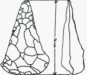Consider a stone axe, as shown in the drawing. Possible attributes for such an object might be:
1. Length in cm.
2. Width in cm.
3. Thickness in cm.
4. Weight in gm.
5. Type of stone. e.g. 'F' = flint.
6. Shape of cross-section. e.g. 'O' = oval or 'R' = round.
7. Shape of point. e.g. 'S' = sharp or 'B' = blunt.
If the length, width and thickness are all measured in the same units, then it is possible to replace variables 2 and 3 with the ratios R1 = width/length and R2 = thickness/length. Then a "round" cross-section should correspond to a very small difference between R1 and R2.

The entries for the data matrix might start out as follows:

 
Axe 1   9.5  0.51  0.39   54.0  F  O  S 
Axe 2  12.2  0.52  0.45  178.0  F  O  B
Axe 3  10.4  0.48  0.48  150.0  F  R  B
 
           and so on

The values of the attributes for each object are recorded in the "data matrix". Typically we may have about ten attributes to be measured for each object and require several hundred objects in the survey. The data matrix will probably occupy one or more notebooks, each page containing 10 columns for the 10 attributes and each row describing one object. The matrix will spread over many pages, as the objects are recorded. Collecting the data is usually the most tedious part of any classification, but accurate data is essential if the resulting analysis is to mean anything at all.

Data Verification.

It is never possible to check that the correct values have been typed into the computer, only that the data is in the correct form for that variable. For example, if a numeric variable was 56.25 and you typed 56.52, both values are probably within the required range of values for that variable and so there is no form of verification which can detect this. The nearest we have is to arrange that all the data is typed in by two or more researchers, working independently, and then compare the data matrices to see whether they agree. Even this duplication is no use if the value was incorrectly written down in the original notebooks.

Automatic methods of data recording can avoid some of the more common human errors, but often have their own problems. Although measuring the same variables for several hundred objects is a tedious and repetitive job and not one which makes it easy to retain interest and concentration, it is vitally important to get these values measured and entered into the computer with the maximum care and accuracy. If the data is wrong, all the resulting analysis is a waste of time.

1. Numeric Data.
The computer program to accept the input data can check that this is a real number lying in the correct range. Some sets of data have patterns which can also be checked, but in general the range of allowable values is the only thing which can be checked.

2. Ordered Multistate Data (or Integer Data).
The input must be an integer value, lying in the correct range.

3. Binary Data.
The input must be 0 or 1. Sometimes presence/absence data may be coded as p and a and then the input program must convert p to 1 and a to 0. Similarly, if the answers in a survey are yes or no, then y = 1 and n = 0. Sometimes the data is not independent, we may know from the context that a "yes" to question 3 must always correspond to a "no" for question 16, and when this is so, we can write the validation program to check for this.

4. Unordered Multistate Data.
Here the input must be one of a number of permitted codes. This may correspond to the use of a CASE statement in Pascal. It is easy to check that the data value is permitted and require an alternative input if it doesn't match. However the choice of codes must be designed to reduce the likelihood of errors. For example, if 'b' meant 'blue' and 'n' meant 'black' or 'noir', then the program is unlikely to detect when newcomers type 'b' and mean 'black'. Sometimes the context may allow the program to query an unlikely value, for example black is more likely as a colour for fruit than for flower-petals.

One special case of unordered multistate data occurs in applications where the data may be incomplete. In this case, the binary presence/absence data becomes ternary data because we must include the three possibilities present/absent/missing. Early work on biological classification ignored this problem because there was no shortage of data and if one plant had no flower to measure, the researchers merely moved to another one which did. Later work in areas such as archaeology had to tackle the problem of missing data because they were working with whatever artifacts had survived and if the incomplete objects were omitted there wasn't enough data to carry out a classification. Thus if a classification of a particular type of pottery was required, we may have presence or absence of a handle as one variable and others related to decoration on that handle. A pot whose surface is smooth and has obviously never had a handle should record this as "absent". One with a handle obviously records it as "present". One with marks on the surface where a handle has been broken off will record this as "missing" and this must be allowed for in similarity calculations. Also all variables relating to decoration on the handle must be recorded as "missing", otherwise the data implies that only undecorated handles get broken. This is not correct. Usually there is no correlation between presence/absence of handles and decoration but in a few cases the form of decoration involves punching holes in the fabric, which weakens the handle and so makes the decorated handles more likely to break off than the undecorated.

Natural Taxonomy.

A "natural taxonomy" is a general classification which may be used by all researchers under all conditions. More restricted classifications, which only apply under certain specific conditions, may be called "local" or "arbitrary" classifications. Because of the restrictions, an arbitrary classification may need only a few measurements to identify an object as a member of a particular group, but the same restrictions imply that the taxonomy is of limited or temporary use. A "natural taxonomy" is sometimes assumed to describe a taxonomy which exists in the data and is discovered by the classification process while an "arbitrary taxonomy" is assumed to be man-made and of limited duration. Whether you agree with the underlying philosophy or not, the terminology may be used to indicate the difference in scale between various classifications. One important result of this is the basic assumption which is implied in most discussions of this topic, namely:

ALL ATTRIBUTES HAVE EQUAL WEIGHT IN DETERMINING TAXA OR CLASSES.

This has certain important results. Firstly it implies that all attributes should be independent - to take a trivial example if we included ‘height in inches’ and ‘height in centimeters’ as two different attributes, then obviously the attribute height is counted twice and has a larger effect on the resulting classes. This assumption also rules out any of the many methods which could be developed giving different weights to the different attributes when calculating the similarity. Finally, it suggests that we should normalise the ordered data in some way so that the magnitude of the numbers does not give more weight to the contribution from a few of the attributes.

When we come to identification, this assumption may not be desirable. Some attributes may be much quicker and easier to measure than others, and a taxonomy which allows quick and easy identification has obvious attractions in everyday use. It is necessary to strike a balance between idealism and convenience.

Definitions.

Phenetic Relationship.
This is the most common relationship in computerised taxonomy, indeed the other possibilities are usually later interpretations of a phenetic result. It is based solely on the overall similarity between objects, although different methods of calculating similarity may lead to minor variations in the resulting classes.

Cladistic Relationship.
This is based on similarities between the actual objects here today and a known or hypothetical ancestor. It is often used in studies of evolution.

Chronistic Relationship.
This seeks to place the objects in a time-sequence. Frequently the results of ordering methods are interpreted as chronistic relationships, although some additional information is needed to say which end of the sequence corresponds to the earlier time.

Attribute-space and Individual-space.
Attribute-space has n-dimensions, one for each attribute, and contains t-points, one for each object. The n values in the data-matrix may be considered to be distances along the mutually-perpendicular axes in attribute-space. Since t is very much larger than n in most cases, we usually develop methods in attribute space, and many methods attempt to reduce A-space to 2 or 3 dimensions so that the points may be plotted and examined visually.
Individual-space has t-dimensions and n points and is usually less convenient to handle and visualise.

Types of Groups.

1. Monothetic Groups.
Each member must possess all the attributes which define the group. This means that identification is quick and easy - you simply move down the tree structure, branching on the value of each attribute in turn, until you finish up with the desired group. This is particularly easy when all the attributes are binary. One example of such a grouping is the identification of flowering plants in a flora.

It has the major disadvantage that if one attribute value is missing, it is not possible to continue down the tree and complete the identification.

2. Polythetic Groups.
No attribute is essential for membership of the group, but each member must possess the majority of the attributes. Some will probably possess all the attributes and others will have different ones missing.
Identification assigns a new object to the group to which it is most similar. In order to calculate this, we must have an object or a list of attribute values for each group. The new object is compared with each of these definitions in turn and the similaritiesare calculated.

1. Average Object or Centroid.
This may be used for numeric attributes. The value for each attribute is the average or mean value of that attribute calculated over all the objects which defined the group. It is not recalculated as new objects are added to the group. It need not correspond to an actual object, though it will be close to many of them.

2. Median Object.
This may be used for unordered (or binary) attributes. The value chosen for each attribute is the commonest value for that attribute.Again it need not correspond to an actual object .

3. Centrotype.
This is the object in the group whose average similarity to all other objects defining the group is the highest. This definition must always give at least one actual object, the "type specimen", to define the group.

Frequently objects are defined by a mixture of types of attribute and then either the centrotype or a mixture of mean and median objects must be used to obtain the definitive list of attribute values for each of the groups.

Reading and Exercises.

1. During the next week, each evening think carefully about the conversations you have had during the day and list examples of the times classifications have been used to discuss everyday objects. Which of these are assumed to be `natural taxonomies', where the assumption is that everyone will be using the same assumptions and terminology and which are obviously temporary classifications, assumed for a particular short-term need ?

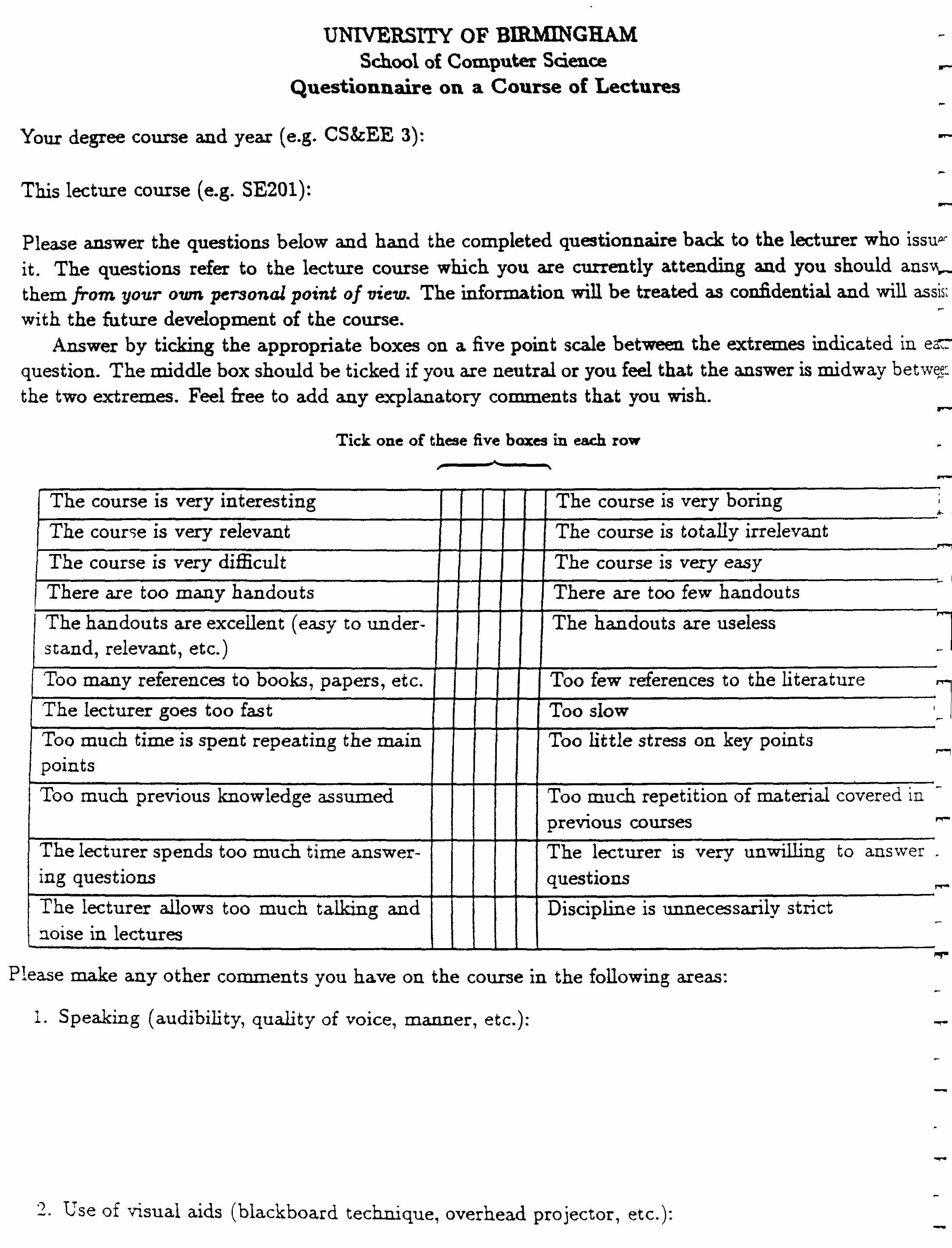
2. Each term questionnaires are handed out for the different courses and for the M.Sc as a whole. They serve many purposes, but one of these is a need to classify the courses into "satisfactory" and "unsatisfactory" and hence to concentrate on improving the unsatisfactory ones. (Note that this is a long-term process and responses in one year are unlikely to produce improvements in that year.) If this were the sole purpose of the questionnaire, how should it be designed? A copy of the questionnaire is included in this booklet, you should study it and consider how the assumption of computer analysis would require changes to the questions to be answered.

3. Borrow the copy of "Numerical Taxonomy" by P.H.A.Sneath and R.R.Sokal and read chapters 1, 2, 10 and 11. Make notes of the points covered and decide how far they apply to your own personal position and motives for taking this course.