Introduction.

Copyright (c) Susan Laflin. August 1999.

This text is concerned with the theory underlying the many CAD (Computer-Aided Design) packages currently available. These packages are many and varied in both their scope and their applications, but they have some things in common. They are all concerned with the storage and manipulation of curves, surfaces and solid objects within a computer.

When we come to describe an object, we may use words or we may indicate shapes, either by drawing on paper or by hand-waving to indicate the outline. In order to store the same information in a computer, we must translate these ideas into numbers and equations. The result may be a drawing on the screen, which may then be edited as required, but within the computer it must be expressed mathematically.

Many of the problems with human-computer interaction arise because of the different way in which the data are handled. The human can look at the object as a whole and describe it in terms of colour and shape. The computer must work in terms of numbers, and requires the shapes to be described as mathematical equations. It can never "look at the shape as a whole" but only apply clearly-defined tests to each point, one at a time.

One of the main problems is the large amount of information needed to describe even the simplest shape. In general, we can either type in vast quantities of data and use very simple equations to interpolate between the points or input a comparatively small amount of data and use more complex equations to derive the objects from these. This course will discuss some moderately complex mathematics in order to reduce the amount of data needed.

Approximation.

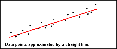
When we have a large amount of data and we wish to replace it with a single line or curve, we need to use some method of approximation. This requires finding which one of a family of similar curves gives the "best fit". To find this best fit, we need some method of calculating the coefficients of the curve which will minimise the distance between all the points and the curve.

This is usually achieved by calculating the "norm of the error function" and deriving conditions to minimise this. The choice of the norm used will define the method and different norms will lead to a slightly different curve for the "best-fitting function". Two norms in particular have been widely studied and there is much software available which uses these to fit a variety of curves.

Reference: "Approximation Theory and Numerical Methods" G.A.Watson. Wiley 1988

The first of these is the L2 norm , which results in the "least-squares" method . This method should only be used for linear regression, since it becomes extremely unstable for higher order polynomials.

The second is the L-infinity norm , which results in the "minimax" method . This is much more stable, but is a comparatively recent method which has no analytical solution and can only be solved using a computer-based iterative method. The "second Remez algorithm" is a good way of implementing this method.

Reference:Open University course M351 "Numerical Computation" Units 9 & 10.

Interpolation.

Interpolation assumes that the data points are accurate and are supplied in the correct order. It fills the gaps between them by joining the points by a set of curves. If the choice of interpolating curves is a good one, the resulting output gives the impression of a single smooth curve over the defined interval.

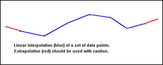
The polyline function gives piece-wise linear interpolation. This is very fast and does not add any extra maxima or minima to the curve, but if the change in slope from one interval to the next is great, then the polyline will give an unpleasantly jagged appearance. Most of the methods involving higher order curves have been developed to provide a "polysmooth" output and of these, the "cubic spline curve" is very widely used.

Once curves have been obtained for the interval over which the data has been provided, there is a temptation to extend the curves on either side (extrapolation). Although tempting, this should be used with caution since there is no information available about the values outside the data interval and extrapolated curves can be very misleading.

Piecewise Linear and Cubic Interpolation.

This section discussed the early development of methods of piecewise interpolation over a set of data points. It covers: Linear (polyline) interpolation; the use of parabolic blending to give a form of cubic interpolation; the Hermite method for cubic interpolation and several examples (Simple Hermite, Bessel, and Akima methods).

Spline Interpolation.

This section covers general spline theory and particular examples of spline fitting such as cubic and quadratic splines.

Curves defined by control points.

A general discussion of the approach used in Computer Aided Design to define curves by means of blending functions and control points. These methods include hat functions, Bezier and B-spline curves and NURBS (Non-Uniform Rational B-Splines).

References.

1. Numerical Computation Williams.

2. Foley et al chapter 9.

3. Rogers and Adams chapters 4 and 5.

4. Rooney and Steadman chapter 7.