Copyright (c) Susan Laflin. August 1999.

Piece-wise Linear Interpolation

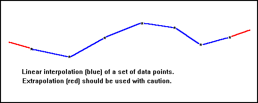
This is a very simple idea, but there are still many occasions when it provides a sufficiently good approximation. It is fast to calculate and there are no unexpected side effects. It is not restricted to two-dimensions, and the only constraint is that successive values of the independent variable (usually x giving curves of the form y=f(x)) should not be equal.

Each pair of points is joined by a straight line. So the line joining [x1,y1,z1] to [x2,y2,z2] is given by the equations:

(y-y1)/(y2-y1) = (x-x1)/(x2-x1)

and

(z-z1)/(z2-z1) = (x-x1)/(x2-x1)

The first equation may be re-written in the form

(y - y1) = (x-x1)*(y2-y1)/(x2-x1)

which will give correct results for all values of y, even when y1 and y2 are equal in value.

Parabolic Blending

Reference: Rogers & Adams section 5.7 for a more detailed discussion.

To understand this method, let us consider a set of points P0, P1, P2, ..... , Pn through which we wish to interpolate a smooth curve. Consider a section part way along this set, say P3, P4, P5, P6 and assume that we have fitted one parabola P(r) to the points P3, P4 and P5 and a second parabola Q(s) to the points P4, P5 and P6. For the interval (P4, P5) where the fitted parabolae overlap, we can blend them together to give a final curve from P4 to P5. This is calculated as follows.

The first parabola P(r) is defined in terms of the coordinate system (r,u) with the origin at the point P3, and r measured along the line P3P5 (taking values r1 at P4 and r2 at P5) and u perpendicular to r. Thus the equation becomes

u = P(r) = k1 * r * ( r2 - r )

The value of k1 is chosen so that the curve passes through the point P4. The second parabola is treated similarly and defined in terms of coordinates s and v. This coordinate system has its origin at P4 and s is measured along the line P4P6 with values s1 at P5 and s2 at P6. The coordinate v is perpendicular to s and the parameter k2 is chosen so that the curve passes through P5.

v = Q(s) = k2 * s * ( s2 - s )

The final blended curve joining P4 and P5 is defined in terms of the variable t, which is measured along the line P4P5 and takes the values 0 at P4 and t1 at P5. This gives the final equation

c(t) = [1-t/t1 ]*P(r) + [t/t1]*Q(s)

At the point P4, c(t)=P(r) and at the point P5, c(t)=Q(s) so this curve blends smoothly into the original parabolae at the end points. The curve c(t) is a cubic and should only be used in the interval P4P5. It does not usually pass through either P3 or P6. To fit the entire curve, similar cubics can be found for all the intervals from P2 to P(n-1), but the two end intervals do not have such curves and should be represented by the single parabolae fitted over these intervals.

The spacing of the points may be varied, so that regions of high curvature may be represented by closely-spaced points giving an accurate representation of the profile. If the frequency of the points is not high enough, additional points may be inserted and the extra curves calculated until a satisfactary profile is obtained. This is particularly useful for CAD applications.

Piece-wise Cubic Interpolation

In an earlier chapter, we discussed the case when a mixture of piecewise linear and piecewise cubic interpolation was used to give a `smooth' curve through a set of points. In this section, we shall discuss the case when a set of cubics are used for this purpose, that is a different cubic for each interval. The conditions at the "knot points" where the curves join ensure a smooth fit which looks like one curve through the whole set of points.

Hermite Interpolation

This is a general method which includes the remaining three methods in this section. For each set of cubics, either y = F(x) or z = G(x), estimates of both the value and the first derivative at each value of x are required. Then the cubic y = F(x) for the interval from x[i] to x[i+1] may be calculated from the four values y[i], s[i], y[i+1] and s[i+1], where s[i] is the value of dy/dx at the point x=x[i]. Since the z-values may be calculated in exactly the same way, they will be ignored in the following discussion. You should remember that all these methods have to be calculated a second time to give the values of z as well as those of y.

Simple Hermite Interpolation

I developed this version of Hermite interpolation as the simplest possible version, for the benefit of those students whose familiarity with mathematical terminology was small. It indicates the method of Hermite interpolation and can be applied with calculating complex sums and products (Besel and Akima) or solving a set of simulataneous linear equations (cubic spline). Some maths is unavoidable, but it has been kept to a minimum.

Consider a set of n+1 points (xi,yi, i=1,2,....,n+1), giving n intervals with interval i going from Pi (xi,yi) to P{i+1}(x{i+1},y{i+1}). A straight line over interval i would join Pi to P{i+1} with the gradient

gi = (y{i+1} - yi)/(x{i+1}-xi)

For Hermite Interpolation, you will need one value of gradient fi at each point Pi. At the two end-points you may choose f1 = g1 and f{n+1} = gn At each of the other points, you will have the join of two linear segments and so it seems best to choose the average

f(i) = 0.5* (g{i-1} + gi )

Let us assume that the equations of the cubic are

y = at^{3} + bt^{2} + ct + d

and

f = dy/dx = 3at^{2} + 2bt + c

If this is used to fit a curve joining the points (xi,yi) and (x{i+1},y{i+1}), then you should choose t = x - xi. At the point (xi,yi), you know that t=0 and so the above equations give

yi = d and dy/dx = c = f(i )

If you define h = x{i+1}-xi then at the point (x{i+1},y{i+1}) the equations give

y{i+1} = a h^{3} + b h^{2} + c h + d

and

dy/dx = f{i+1} = 3a h^{2} + 2b h + c

These last two equations must be solved to give the values of a and b. Multiplying the first equation by 3 and the second equation by h gives

3ah^3 + 3bh^2 + 3ch + 3d = 3y{i+1}

3ah^3 + 2bh^2 + ch = hf{i+1}

Subtracting the second equation from the first one allows you to calculate b

b = (3y{i+1} - h f{i+1} -2ch -3d)/(h^2)

Once b has been calculated, you can substitute it in the second equation to obtain the value of a

a = (f{i+1} - 2bh -c)/(3h^2)

This means that the cubic joining P{i} to P{i+1} has the equation

y = a(x-xi)^3 + b(x-xi)^2 + c(x-xi) + d

for values of x from xi to x{i+1}. It will then be necessary to calculate several small segments for each interval and probably use a separate call to Polyline for each interval in turn.

Bessel Interpolation

This uses three points, x[i-1], x[i] and x[i+1] to estimate the value of s[i]. Thus the method loses one point at each end of the array. The equation for s[i] is given below, and is equivalent to fitting a quadratic through the three points and using its equation to estimate s[i].

s[i] =((x{i+1}-x{i})^{2}*(y[i-1]-y[i])+(x{i}-x{i-1})^{2}*(y{i}-y{i+1}))
      ---------------------------------------------------------------------
         (x{i+1}-x{i}) *(x{i}-x{i-1})* (x{i-1}-x{i+1})

  This is also a local method. 

Akima's Interpolation

This uses five points to estimate the value of s[i] and so loses two points at each end. It tends to smooth out the curve, which may be desirable, but can sometimes average out kinks in the curve which should be retained. The equation to estimate s[i] is correspondingly more complicated.

If 			d[i] = (y[i]-y[i+1])/(x[i]-x[i+1])
and			w[i] = d[i] - d[i-1] 
then			s[i] = {w[i+1]*d[i-1]+w[i-1]*d[i]} / {(w[i+1]+w[i-1])}

The method was first described in the Journal of the A.C.M., volume 17 (1970) p589-602.