Copyright (c) Susan Laflin. August 1999.

Approximation and Function Norms.

Consider the case where we have been using a digitising tablet to input data points along the curve. The digitiser may be very accurate, recording values correct to a fraction of a millimeter, but even so the data may contain errors due to inaccurate placement of the cross-wires or shakiness of the wrist in following the curve. Whilst you may assume that such errors will never occur in anything you have recorded, it is nonetheless true that you will need to use sets of data recorded by other people which do contain such errors. The following discussion considers what to do in such cases.

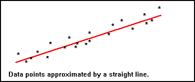
There are two main approaches to this problem. You may smooth the data or you may fit a curve, using one of the well-known approximation techniques. APPROXIMATION provides a curve which need not pass through any of the data points, but which is the closest possible curve to all of them. The order of the points is not important, the shape of the curve is determined by the form of equation chosen and the method finds the "best-fitting" curve according to some criteria. Different criteria give different approximation methods.

Function Norms.

Definition of a `norm'.

Let S be a linear space with elements f, g, x, v etc. If we can define a rule which obtains a single real number from each of these elements and use the notation ||f|| for the number derived from f, then ||f|| is a norm if and only if it satisfies the following three conditions:

1. ||f|| is always greater than or equal to 0 and ||f|| = 0 if and only if f =0 everywhere.

2. || k*f || = |k|*||f|| where k is a scalar.

3. ||f+g|| is less than or equal to ||f|| + ||g||.

The function norm is defined for the space C[a,b] of continuous, real-valued functions over the interval [a,b].

Examples. 
The general Lp norm. 
||f||p = integral from a to b (  |f(x)|^p. dx )^{1/p} 

The L-infinity norm.   
	||f|| = maximum over the interval [a,b]  |f(x)| 

For a general function, a norm may be of interest, but not of immediate use. However, when we come to consider error-functions the applications to approximation are of immediate relevance.

Suppose we have a complex function f1(x) which is very time-consuming to calculate and we note that over the interval [a,b] it is very similar to a much simpler function f2(x). The error function e(x) is given by the equation:

e(x) = | f1(x) - f2(x) |

Usually the approximating function f2(x) includes parameters which may be varied and we would like to find those values of the parameters which give the `best-fit' to the function f1(x). If we are very lucky, it will be possible to find parameters which make the norms ||e(x)|| over the interval [a,b] equal to zero and this will tell us that f1(x) and f2(x) are equal at every point x in the interval. Usually we are not able to achieve this, and have to make do with the values which give the minimum value of one of the norms ||e(x)|| over the interval.

There are many possible norms and each one will give slightly different values for their "best-fitting" parameters. The two most commonly used ones are the L2 norm, giving the "least-squares" methods and the L-infinity norm, giving the "minimax" methods

The theory of approximation is discussed in several textbooks, one of which is "Approximation Theory and Numerical Methods" by G.A. Watson , published by Wiley in 1980. The philosophical concepts which must be discussed when deriving methods for particular norms include the following:

1. Existence of a best approximation.
2. Uniqueness of a best approximation.
3. Characterisation of the best approximation.
4. Construction of methods to determine the best approximation.

As software engineers, we are more interested in practical applications than in theoretical concepts. We note that for the two norms mentioned above, these aspects have been studied and proven and so we may safely concentrate on the last point, the construction of methods to find the best-fitting approximation in any particular case.